Charting Untraveled Paths: The Follow the Gap Method
Introduction
Let’s embark on a thrilling escapade to an alternative to the conventional wallfollowing method, where the standard routine is simply adhering to the left or right boundary of the track. Instead, I introduce you to the ‘Follow the Gap’ algorithm. Its modus operandi is not merely tracing the boundary, but rather, darting through the track, dodging any static obstacles, and strategically finding the best route to circumvent them. Wallfollowing, although useful, faces an Achilles’ heel when encountering distinctively shaped obstacles within the track. That’s where the Follow the Gap algorithm shines. This clever strategist doesn’t require extensive pre-existing data about the track, but rather uses the current situation to make decisions - a trait of its reactive method. Its brilliance lies in overcoming any obstacle without prior map knowledge.
Follow the Gap
Reactive navigation
Reactive navigation is like a skilled chess player, making tactical steering and velocity decisions based on the present sensory input. This method effectively tackles static and, in certain cases, dynamic obstacles.
Gap finding intuition
As the algorithm’s name suggests, the aim is for the car to spot the widest gap in the immediate obstacle landscape and confidently venture into this void to evade a collision. Now, imagine a lidar relaying the following array of distances: [0.2, 6.2, 6.0, 7.0, inf, 3.0, inf, 3.0, inf, 8.0, 1.0, 3.0]. The most straightforward strategy would be to steer towards the furthest obstacle, yet this might not always be feasible. The car might face two obstacles, the distance between which is too narrow for the car to slide through or the turning angle might be physically impossible for the car, as in the case of the 7th element in the given array.
To crack this problem, let’s lay down a working definition of a ‘gap’:
- A gap is a series of at least ‘n’ consecutive hits exceeding a distance threshold ‘t’.
If we apply this definition to the array with n=3 and t=5.0, we find one gap: [6.2, 6.0, 7.0, inf]. Thus, we would steer towards the heart of this gap.
However, this approach isn’t foolproof as the car might be lured to pass between obstacles where it wouldn’t fit. To resolve this issue, we turn to an approach that’s a beloved mainstay in robotics.
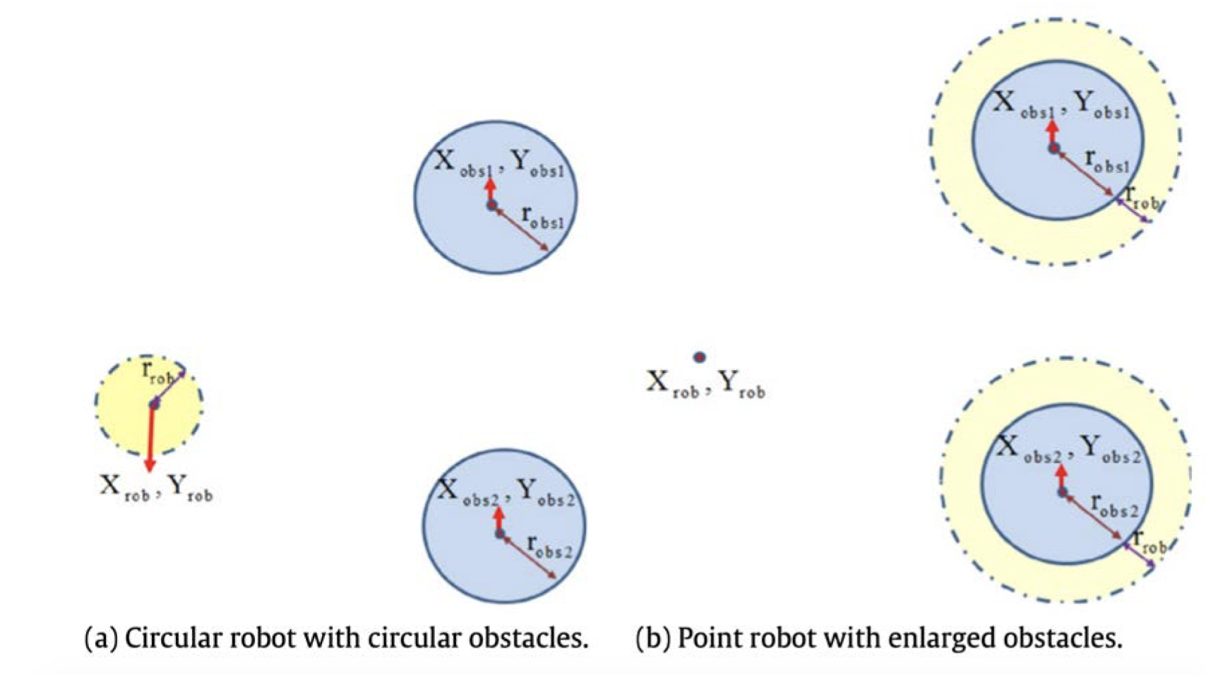
Point Robot Approach
Here’s a neat trick: assume the robot to be circular. With this approximation, we can inflate the obstacles by the robot’s radius. Hence, even if we decide to squeeze the robot between two obstacles, we can represent it as a point object while still ensuring it fits between the two obstacles since we have cleared the path by at least the radius of the robot. A picture is worth a thousand words, and the following figure does an excellent job of illustrating this concept (UV lecture follow the gap):
Disparity
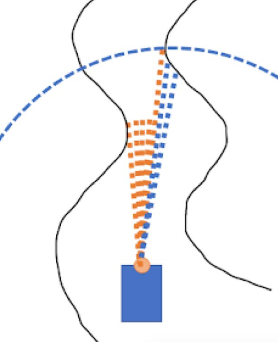
To detect potential gaps, we scan the lidar readings for consecutive readings that exceed a certain threshold. These readings are then masked to appear closer to the lidar. The points that remain beyond this mask are the actual points the car can navigate through. The figure below, from UV lecture follow the gap, offers a great visualization:
Follow the gap algorithm
The steps to follow the gap are:
- Find the nearest LIDAR point and create a safety bubble of radius rb around it.
- Set all points within the bubble to a distance of 0. This can be achieved by computing the arc’s length and determining which points fall within the bubble’s radius rb. All these points are then set to 0.
- Locate the maximum sequence of consecutive non-zeros among the free-space points. This sequence represents the maximum gap for the car to maneuver.
- Find the best point within this maximum sequence.
For optimal results, it’s crucial to detect obstacles at farther ranges early on. Early detection allows for smoother turns, avoiding sharp maneuvers that could reduce the vehicle’s speed.
Disadvantages
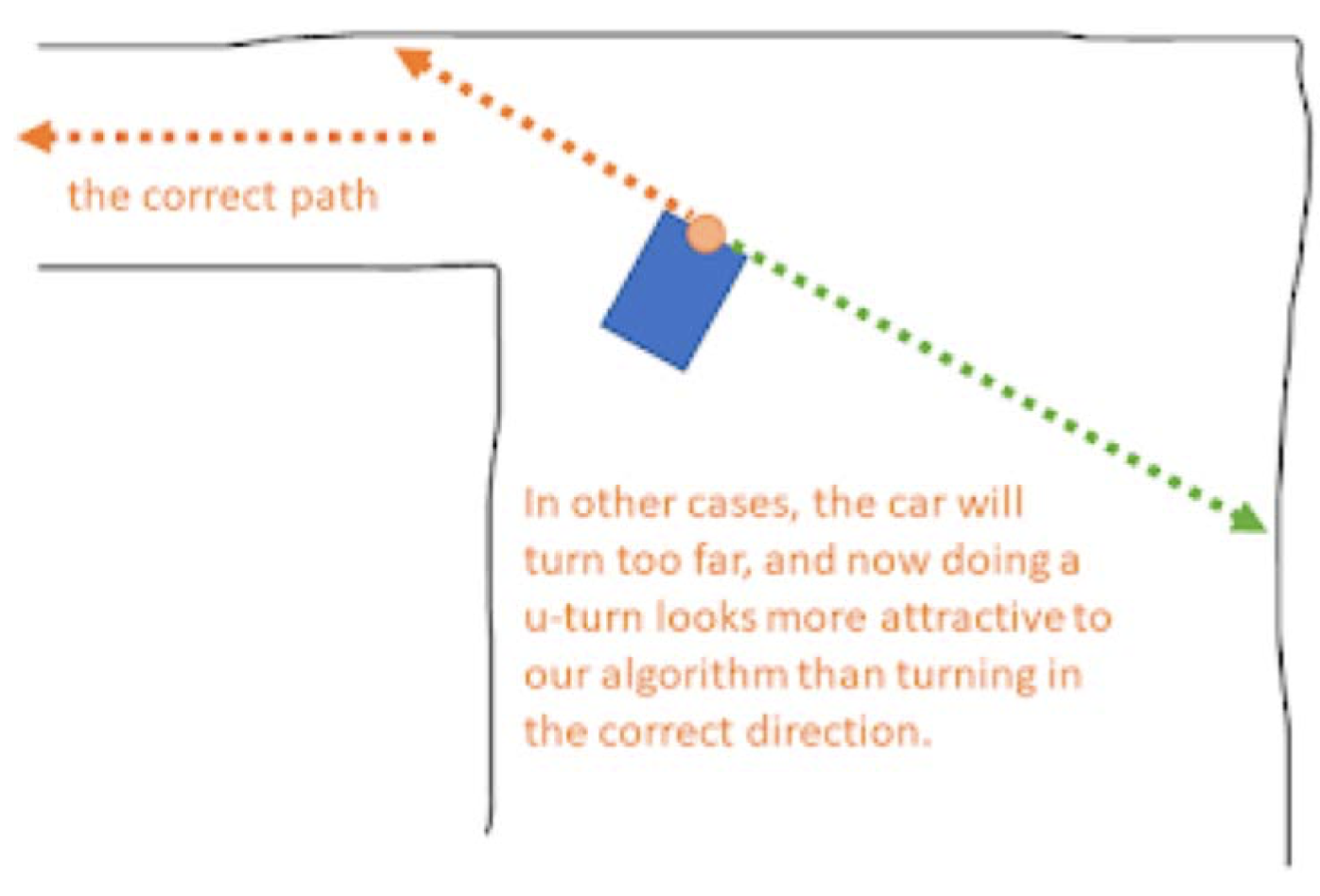
This algorithm isn’t without its flaws. There’s a risk of the car executing U-turns if it’s moving too fast and has to make a 90-degree turn, which it can’t currently see. In such a scenario, the car may perceive a point on the track’s opposite side rather than the turn itself. The figure below demonstrates this flaw:
The video below offers a practical demonstration of the Follow the Gap approach.
F1Tenth Lab4 assignment
My implementation of the Follow the Gap algorithm followed these steps:
- Process each LiDAR scan, considering only a field of view of 90 degrees (45 to the left and 45 to the right, with the 0th degree directly in front of the car). Set each value to the running mean of window 7 through convolution, and clip all values over 3m to 3m.
- Locate the closest obstacle and set all points within a certain radius around it to 0. This is done by computing the arc of the radius proportion and the closest point, then determining all angles inside this bubble. The ranges corresponding to the indices of angles within the bubble are then set to 0.
- Find the max gap by locating the longest non-zero consecutive values in the indices of the processed lidar scan.
- Find the deepest possible scan and steer towards it.