SLAM Unveiled: Simultaneous Localization and Mapping
Diving Into the World of Autonomy
As we steer away from the traditional reactive methodologies, we start to appreciate the power of embedding mapping information in autonomous vehicles. The cornerstone of this approach is a technique known as Simultaneous Localization and Mapping, better known as SLAM. This article will dissect key components of SLAM, delve into the intricacies of Occupancy grid maps, and offer insight into a variety of fundamental SLAM algorithms.
The twin problems of localization and mapping are the heart of SLAM. Localization is about finding our position in a given map, while mapping is all about using the sensors at our disposal to create a map of the environment, given that we know the pose of the car. SLAM takes both these problems, marries them into one, and utilizes the resulting data to estimate the robot’s trajectory while simultaneously mapping the environment. It boasts a significant advantage over wall-following or follow-the-map algorithms because it enables long-term path planning instead of merely responding to momentary information.
Deciphering Occupancy Grid Map
In the realm of SLAM, occupancy can be perceived as a binary random variable, assuming either of two states: Free or Occupied.
In formal terms, we denote it as: mx,y:{free, occupied} -> {0, 1}
An Occupancy Grid map is a sequence of cells, each assigned an occupancy variable, i.e., either free or occupied.
The Art of Occupancy Grid Mapping:
The objective here is to assign a probability to each cell of the grid, indicating whether it’s free or occupied based on the robot’s data. We employ Bayesian filtering for this purpose. It involves examining the prior and recursively updating the probability status for each cell, which necessitates the application of Bayes’ rule.
We also need data from the robot’s measurements to pinpoint the obstacle’s location in the robot’s frame of reference. Hence, the measurements for each cell can either denote free or occupied. This can be perceived as the likelihood of observing a specific measurement given our knowledge about the cells. To articulate this formally:
Measurement model: p(z|mx,y) where z~{0,1} It represents the probability of a measurement ‘z’ conditioned upon our knowledge about the value of ‘m’ (the occupancy random variable) in the occupancy grid.
Our measurement models can be one of the following:
-
p(z = 1 mx,y = 1): TRUE occupied measurement, -
p(z = 0 mx,y = 1): FALSE free measurement, -
p(z = 1 mx,y = 0): FALSE occupied measurement, -
p(z = 0 mx,y = 0): TRUE free measurement.
To amalgamate all these into Bayes’ rule:
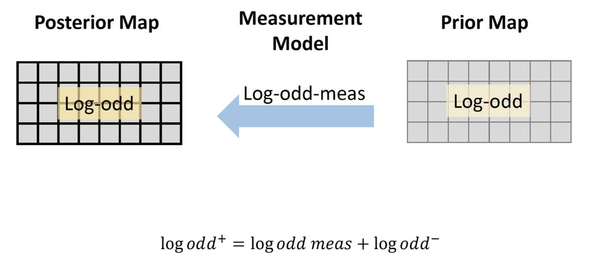
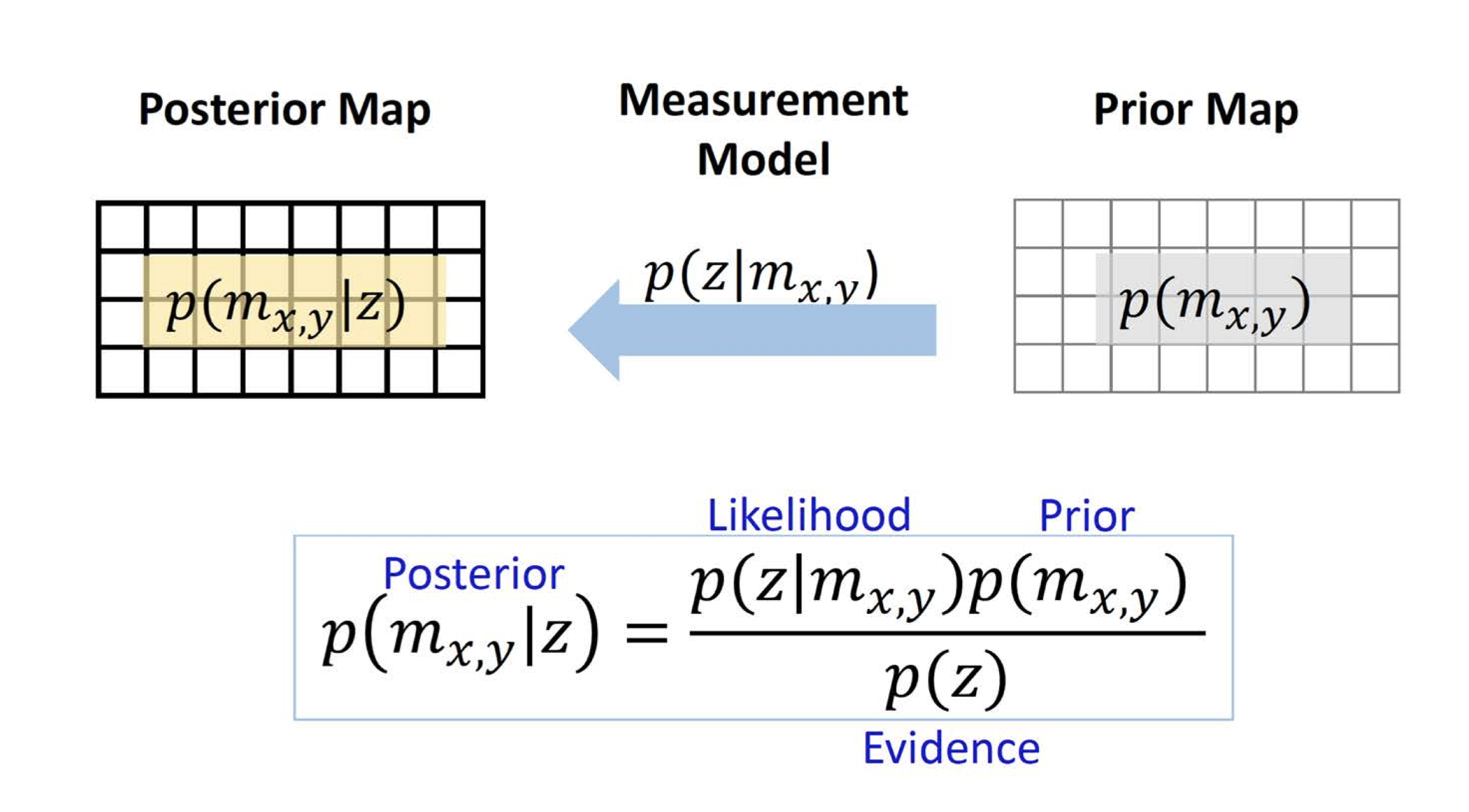 With an occupancy grid (Prior map) at hand, we measure the data from the robot. The probability associated with observing 0 or 1, conditioned on the state itself (measurement model), is used to update our understanding of the occupancy of the grid cell or computing the posterior map (the probability of the cell being occupied or free, conditioned upon what the measurement has reported). The process involves applying Bayes’ rule, as depicted above (ref UV SLAM lecture).
However, dealing with these probabilities can become mathematically cumbersome. A more convenient alternative is working with Odds.
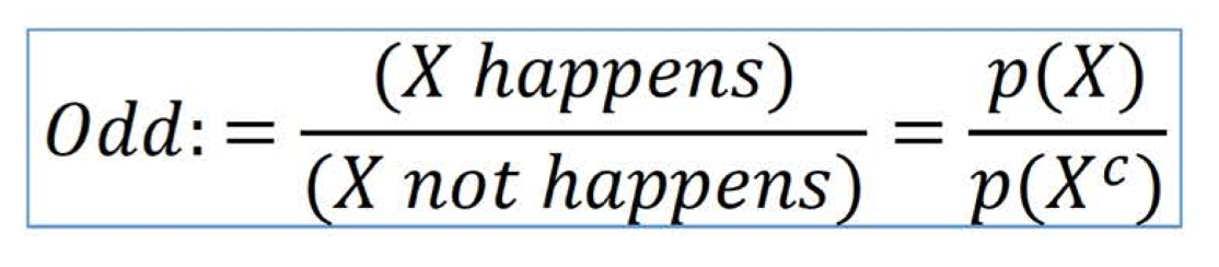 Taking reference from the formula above ( ref UV SLAM lecture), we can see that the odd is essentially the ratio of the probability of X occurring to the probability of X not occurring.
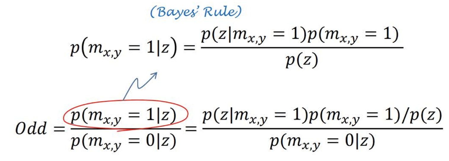
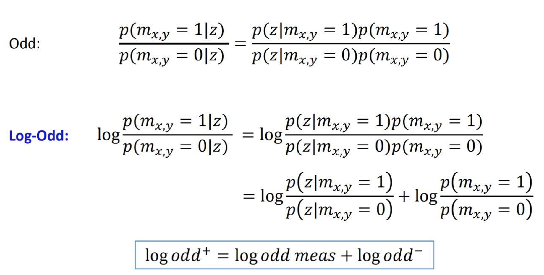
Specifically, the Odd that a certain cell is occupied given ‘z’ is the probability that the cell is occupied given ‘z’, divided by the probability that the cell is not occupied given ‘z’, as shown in the formula below ( ref UV SLAM lecture).
 Applying Bayes’ rule to both the numerator and the denominator:
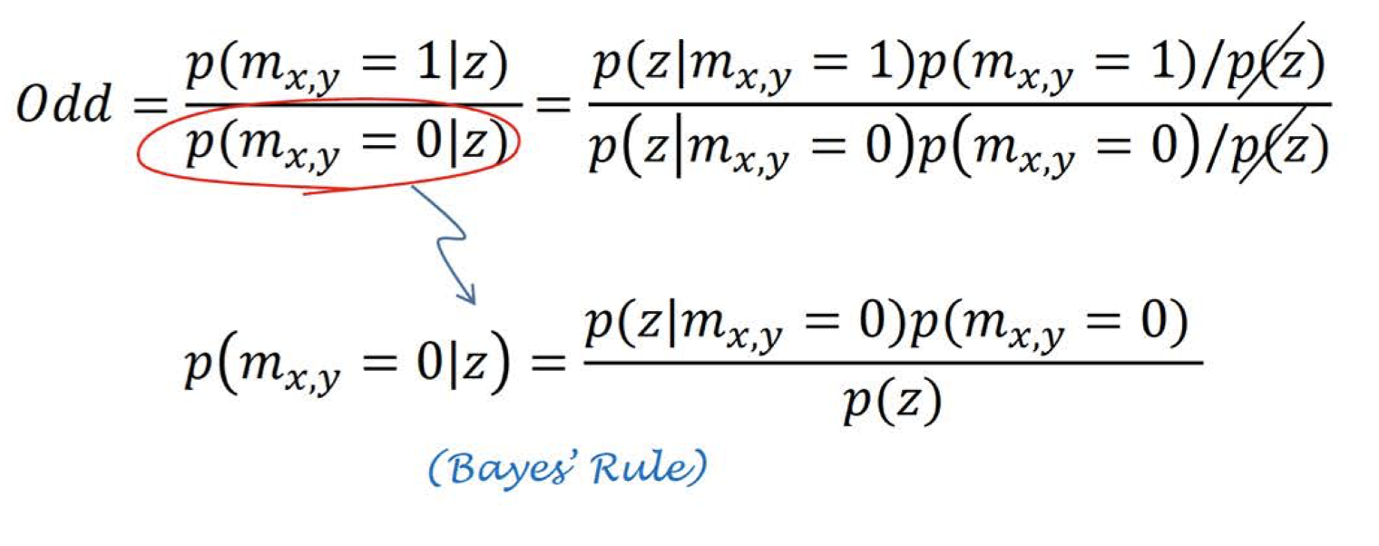 The evidence term p(z) can be eliminated. The resulting equation can then have the logarithm applied to it, leading to a sum of two odds in logarithmic form. This simplifies computations and signifies the same thing as the non-logarithmic version. The formulas shown below highlight this ( ref UV SLAM lecture):
Hence, the measurement model in the log odds version will be:
Remember, every grid cell is updated at each point in time. We also need to consider the robot’s location on the map. The above descriptions consider only a single lidar beam scan, but let’s delve a little deeper. For the next section, it’s recommended to review the previous post on ROS transformations, as it’s required to understand the forthcoming concepts.
Grid-Based Range Measurements
Given a map frame and a base_link frame, let’s assume we receive a measurement along the primary x1 direction, at a distance ‘d’ from the robot’s base link. We’re aware of the robot’s pose at any given time, allowing us to deduce that the reported occupied cell is ‘d’ distance away from the robot’s base link. We can calculate the coordinates of this point and express it in the global frame of reference using the rigid body transformation equation shown below, as explained in the previous post.
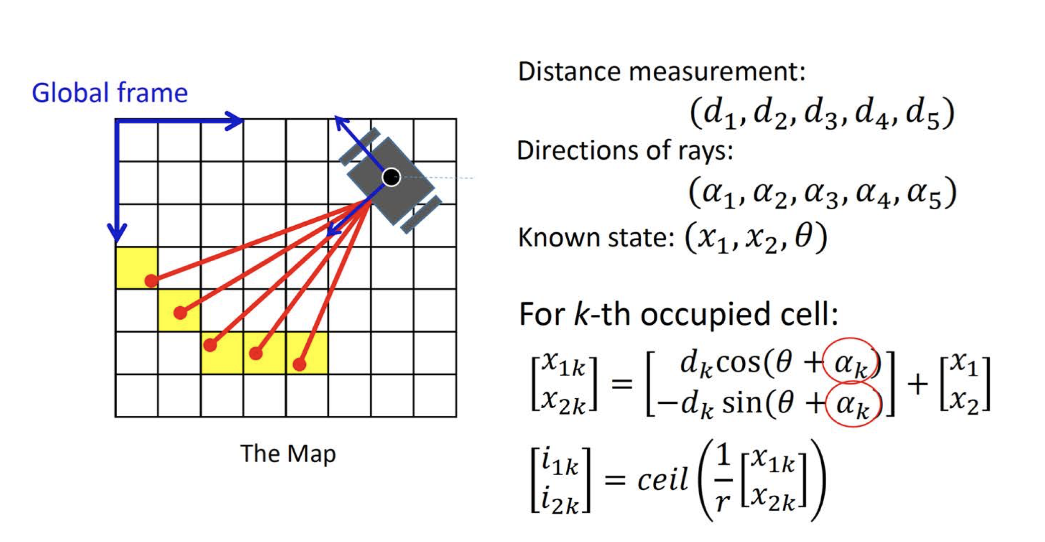
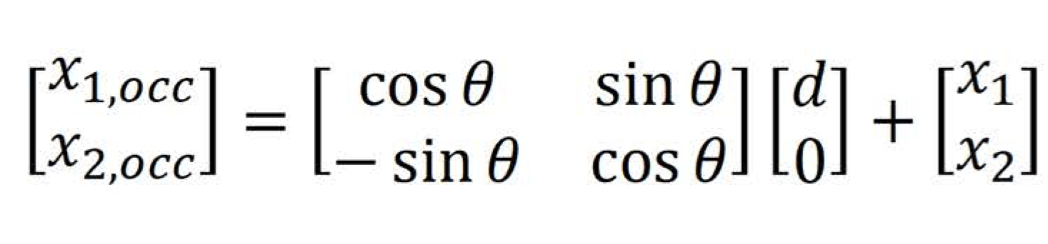 This process is done in continuous space. To convert it to grid space, we need to know the grid’s resolution ‘r’, and then we can place the point in grid ‘i’, where i = ceil(x/r). Because we have x1 and x2, we need to calculate both i1 and i2. Since the robot provides multiple measurements at any given time, not just one, we also need to consider αk, which represents a single lidar beam of the robot. This process is vividly illustrated in the image below ( ref UV SLAM lecture).
Google Cartographer: An Overview
This algorithm particularly excels in a segment of SLAM called loop closure, efficiently reducing computational requirements.
Loop Closure: The What and Why
Over time, errors accumulate as the robot updates grid map measurements, causing