Mastering Scan Matching
Introduction
In our previous discourse, we delved into the intricacies of Simultaneous Localization and Mapping (SLAM), shedding light on a unique localization methodology. As we continue our voyage, we will steer towards an alternate approach to localization—employing a time-series of range measurements, colloquially known as scan matching.
Remember, localization refers to determining a robot’s state relative to the surrounding environment. Traditional methods rely heavily on odometry, which estimates the robot’s current pose based on a known starting point and integrated control and motion measurements. Alas, with time, small errors accumulate, causing an increasing uncertainty in pose estimation. To combat this, we introduce range sensor measurements as a solution, bringing us to the concept of scan matching.
Problem Formation
Imagine we have a robot within an environment dotted with landmarks—A, B, C. At time t=0, the robot performs a scan, gathering measurements that quantify the distance from itself to these landmarks in its local frame of reference. As the robot moves in an unknown direction, reaching t=1, these distances naturally shift. We then measure these new distances and aim to discover the transformation ‘R’ that minimizes the difference between the two sets of points. This transformation reflects the movement of the robot, as depicted in the following illustration. [^1^]
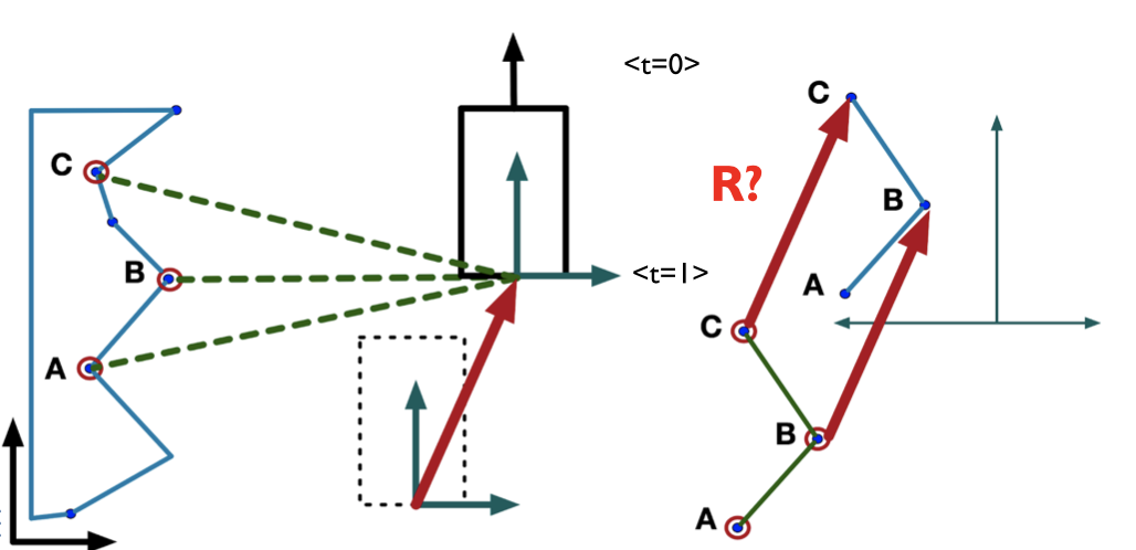
Unfortunately, we can’t precisely identify landmarks A, B, C from the scan readings alone. We are forced to assume the nearest points correspond to each other (correspondence match) and then iteratively seek the most accurate transformation ‘R’.
Iterative Search for Optimal Transformation
- Start with an initial guess for ‘R’
- For each point in the new scan (t=k+1), find the closest point in the previous set (t=k) — this is the correspondence search
- Make a better guess for ‘R’
- Set the new guess as the current guess and repeat steps 2-4 until convergence
Despite its efficacy, the Iterative Closest Point (ICP) algorithm may be slow to converge, and the choice of the initial guess is paramount to its performance. To improve efficiency, we introduce an enhancement—Point-to-Line Iterative Closest Point (PL-ICP).
Point-to-Line Iterative Closest Point
Unlike its predecessor, PL-ICP adopts a point-to-line metric instead of point-to-point. While the latter measures distance to the nearest point on the segment, the former gauges the distance to the nearest line containing the segment. This results in faster convergence as the level sets approximate the surface more accurately, leading to a more precise error approximation. This method achieves a quadratic convergence rather than linear, thanks to the contours of the level being linear and not centered around the projected point.
PL-ICL Algorithm
At t=k:
- Use the previous guess q_k to transform the coordinates of the current scan into the frame of the previous scan.
- For each point, identify the closest line segment (correspondence search).
- Update transform: a. Formulate a point-to-line-error objective. b. Find the transform qk+1 that minimizes the objective.
PL-ICL also employs clever “tricks” for correspondence match search. It performs local search with early termination and a jump table for each scan point.
More extensive research on PL-ICL is necessary for a comprehensive understanding of the method.
For a deeper grasp of this algorithm, I highly recommend Andrea Censi’s original paper, 2008 ICRA-PLICP.
F1Tenth Lab5 Assignment
The final package required for the assignment can be accessed below.