Reading notes: Model-free detection and tracking of dynamic objects with 2D lidar, Wang et al.
Mentioned in post before, the goal of the project is to implement algorithm mentioned in the paper from Wang et. al. The paper focuses on creating framework that estimates and determines what is static background as well as movement of dynamic objects.
The algorithm itself can be divided into several parts. Firstly the new laser and odometry measurements coming from car need to be processed. The process of laser measurement consists of first cleaning the states which is mentioned very briefly in the paper and from my understanding, this means that all points from the previous measurement which are no longer in the LiDAR’s field of view, should be dropped. The authors do not provide any reasoning for this but my guess is that it’s due the easing some of the memory requirement as we do not essentially need to work with anything which we can’t see. One of our own modification during cleaning the states is also drop all points in the memory which are beyond certain threshold. This threshold is chosen to maximise the distance to which we want to detect dynamic object, but at the same time minimise the memory requirement as the assumption at the moment is that the whole framework needs to run in real-time to be usable, which can be hard to achieve with too many “memorised” points. This process is followed by forward propagation, where the motion part of all dynamic tracks according to an appropriate motion model is predicted. This motion model is required, due the main objective of the algorithm, to not have any assumption about the object class (therefore it’s expected motion pattern). This steps is followed by association and update of dynamic and static object measurements finalised by merging tracks which correspond to the same class (static or specific dynamic track). The basic idea of the algorithm is outlined in following figure

As mentioned already the main benefit of this approach is that it allows us to track objects without having to know any informations about the object beforehand. Let’s describe each step more into the detail to understand more details about the algorithm.
Sensor pose prediction on odometry measurement
Individual laser scan beams and a set of odometry measurements are used as input to the algorithm. Without odometry information, the system would not be able to distinguish static objects as all motion estimates are relative to the LiDAR sensor. Odometry information provides us with an estimate of speed v of non-holonomic vehicle, mean angle θ of front wheels.
Dynamic object motion prediction
When new measurements are received, currently existing dynamic tracks are predicted forward using generic motion prediction model before they are updated with the newly received scans. We assume a constant velocity model, because we do not know any information about the object and thus it’s motion pattern. This is disadvantage of working with model-free assumption. We also model not only constant linear velocity component, but angular velocity component as well. This should make motion prediction model able to capture a full range of 2D rigid body motions.
Hierarchical data association
It is not possible to directly observe all state variables in the joint state and for those which we can directly observe, more specifically boundary points belonging to static or dynamic object, it is difficult to tell which one do they belong to or if it is a new boundary point, which haven’t been seen before. Each time we get new set of LiDAR scan, we have to determine following:
- If new measurement is a part static object:
- Is it already existing boundary point?
- Is it a new boundary point?
- If new measurement is a part of existing dynamic object:
- Is it already existing boundary point on the object? If that’s the case it also needs to be determined which specific object this measurement belongs to.
- Is it a new boundary point on the object?
- Is new measurement part of new, yet unassociated object?
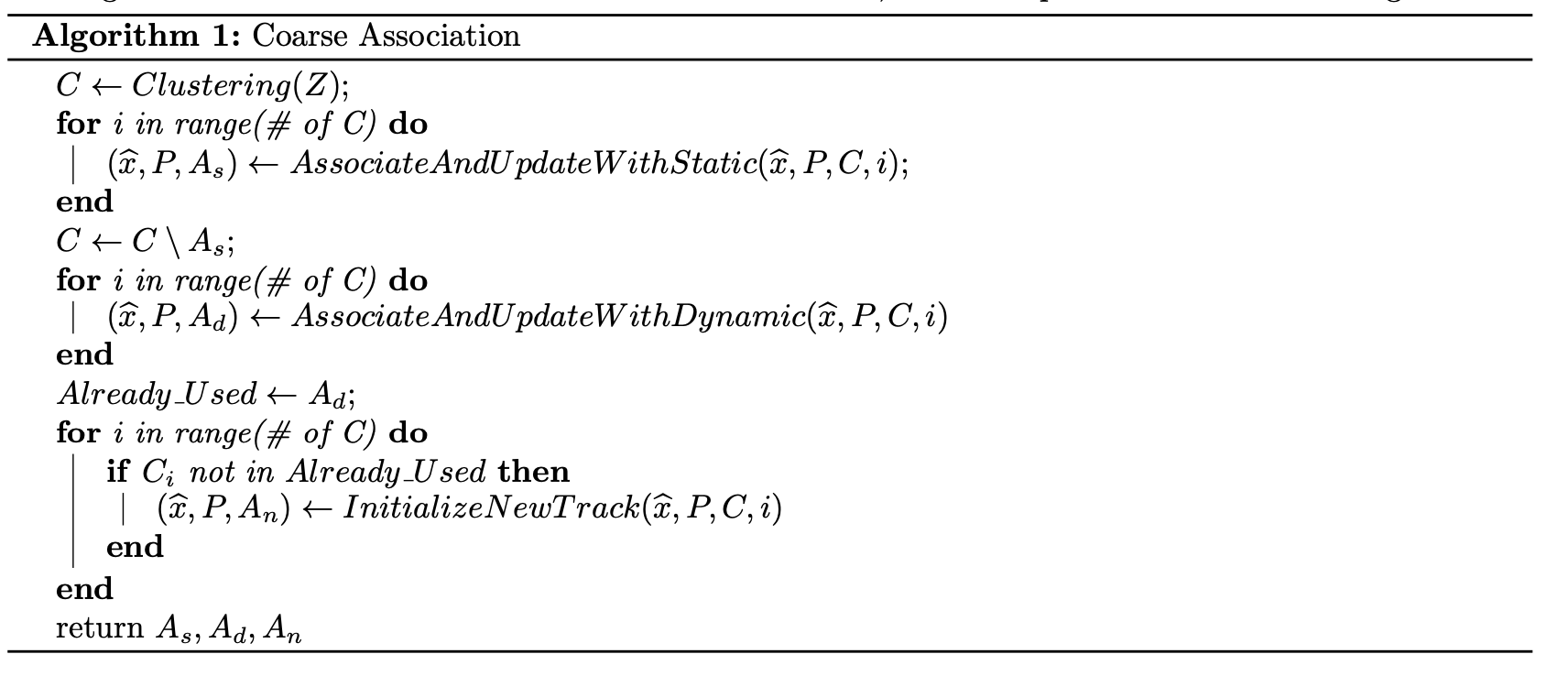
In order to solve data association problem we have to associate the measurements on low and high level. Meaning, on high level we want to firstly create rough associations on coarse scale, where we divide all newly observed measurements into clusters and find out for each cluster if it belongs to already existing static background or dynamic object. If neither is the case than we assign it as a new, yet unobserved object. On low level we create fine associations, where the each measurements within each cluster is either associated to yet exiting boundary point or used to initialized a new point.
Coarse-level data association
In the previous section we discussed that in order to decide if the new set of measurements belongs to boundaries of already existing objects or if the measurements are new objects, we need to break down the problem into coarse and fine level association. We mentioned as well that in coarse association we want to divide incoming measurements into clusters. More specifically, we divide incoming laser scan data into set of clusters C = {C1, C2, …, C|C|}.
Using ICP, we align the incoming lidar scan with clusters which already has been associated to static background. After that, we calculate a transformation between the corresponding points: if the transformation (either its translation magnitude or rotation magnitude) is too large, then the association is rejected and the cluster deemed to not be a good match with the candidate object. Associated clusters that are assigned static background are removed from the set of clusters C. Then, we repeat the same procedure on the remaining clusters in C, however this time we are trying to match incoming clusters with already known dynamic objects using ICP.
The rough coarse association algorithm is visualised in pseudocode bellow.
Fine-level data association
While coarse-level data association helps us identify which clusters of LiDAR points are associated with which objects (and which ones are possibly of new objects), in order to update the state of our currently tracked objects, we need to perform point-to-point matching. Successfully performing this matching is critical to the entire system, since we use these matches to estimate a transformation that is used to update the state of our tracked objects.
Track initialization and merging
During each LiDAR update iteration, we check to determine whether or not any currently tracked object is either part of the static background, or part of another dynamic object. In this, we diverge from original paper and check all objects, rather than just the ones newly initialized. We find experimentally that this allows the algorithm to correct previous mistakes by merging tracks that were previously, and mistakenly, not merged. To perform the merging step, we calculate the Mahalanobis distance between each track’s state and the merging target’s state, taking into account the track’s covariance. We first test to see whether or not each track should be merged with the static background by comparing the track’s velocity with a proposed value of 0 (static objects have a velocity of 0). To determine whether or not a track is part of the static background, we compute the Mahalanobis distance between the track’s velocity probability distribution and 0, and compare the distance against a chi squared significance value. If the distance is lower than the chi squared value, then we merge the track with the static background. The remaining tracks are then tested against other dynamic tracks to see whether or not they should be merged. The merging procedure works here nearly the same as the procedure for the static background: rather than comparing the track’s velocity, however, we compare the track’s position and velocity against the proposed merge target’s. If the calculated Mahalanobis distance between these two distributions falls below the chi squared significance value, then these tracks are merged.