Joint Compatibility Branch and Bound algorithm

Joint Compatibility Branch and Bound

While coarse-level data association helps us identify which clusters of LiDAR points are associated with which objects (and which ones are possibly of new objects), in order to update the state of our currently tracked objects, we need to perform point-to-point matching. Successfully performing this matching is critical to the entire system, since we use these matches to estimate a transformation that is used to update the state of our tracked objects.

In fine-level data association, we perform such matching. The core algorithm in this stage is the Joint Compatibility Branch and Bound (JCBB) algorithm, a common algorithm used for MOT (multi-object tracking) data association. In the JCBB algorithm, we run a depth first search to find a joint data association that minimizes jNIS (the joint normalized innovation squared). The formula for jNIS is as follows. Say we have a set of measurements z_σ that we propose are associated with a set of currently estimated boundary points h_σ. The joint pairing has an innovation covariance of:

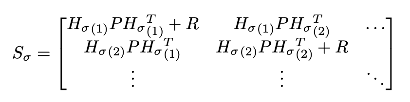
Where P is the covariance of the track, R is the expected measurement noise of the LiDAR, and Hσ is the Jacobian of the measurement model of the boundary points. Then, the jNIS is:

jNIS = (z_σ - h_σ)^T S^-1_σ(z_σ - h_σ)

This formula is similar to the Mahalanobis distance, which measures the distance between two probability distributions.

Implementation

The JCBB fine association algorithm is comprised of three parts. First, we construct an initial association based on the output of coarse association– scan points and estimated boundary points that are sent into an array to form our initial association. Individual Association: For every scan point, and every estimated boundary point, we then compute their potential individual compatibility. This allows the later Depth First Search to operate efficiently, by pre-rejecting incompatible points (typically ones that are far away from each other). The initial association is then pruned based on these individual compatibilities. Prune Association: We also wish that our output association has a one-to-one pairing between bound- ary points and scan points. That is, each scan point can only be paired to at once one boundary point, and each boundary point can only be paired to at once one scan point. Thus, the initial association is further refined to remove double-pairing – in cases where two scan points are paired to one boundary point (or vice versa), we simply clear the association for both points.

Minimal Association: Then, we run through the association, and iteratively remove pairs from the association to yield the largest jNIS decrease. We continue doing this until the total jNIS of the association falls below the chi squared significance value. In practice, this operation is computationally expensive (it requires lots of iterations), so we cut this portion of the algorithm off if the number of iterations exceeds a max iteration parameter.

Depth First Search:

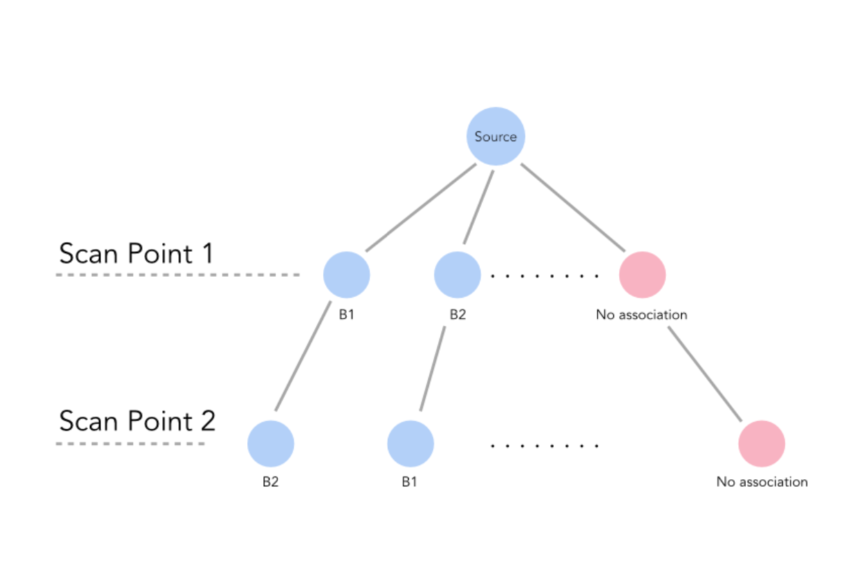
With our minimal association, we begin adding points to the association to generate a valid association (one whose jNIS falls below the chi squared significance value) with the maximum number of pairs. If there are multiple associations with the same number of pairs, we choose the one with the lowest jNIS value. In practice, we implement this portion of the algorithm as a depth first search. A diagram of a sample search tree is shown below. As can be seen, each level of the tree refers to a scan point – as we go through the tree, we search through sets of boundary points that are associated with our scan points. Every level of the tree has an option for its scan point to be associated with no boundary points, in which case it becomes associated with a ”nAn” (the red circles in the below plot). At every point in the tree, we recalculate the jNIS of the proposed association thus far.

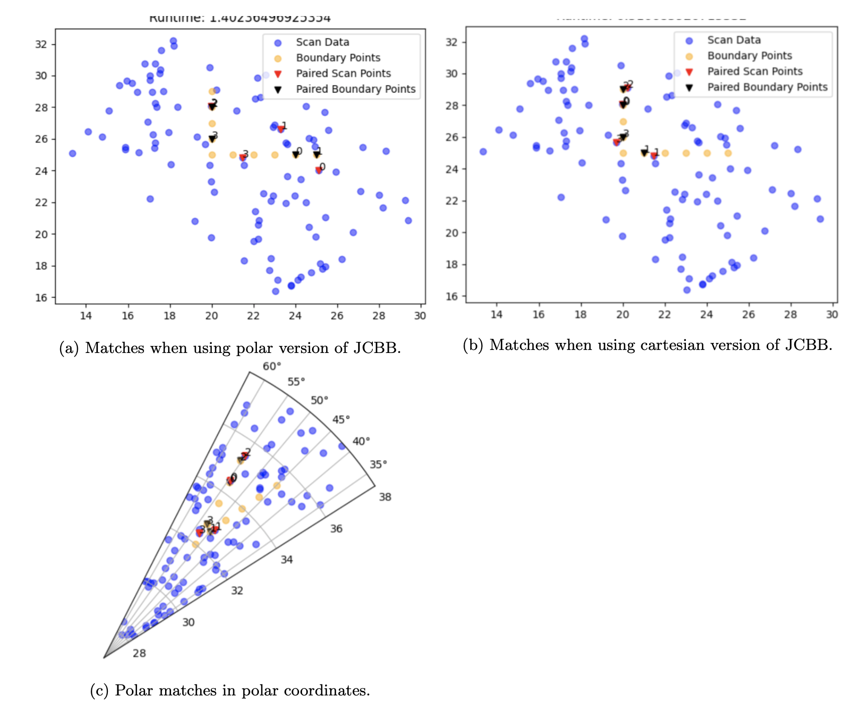
To improve the efficiency of the DFS search, we prune portions of the tree. jNIS is a monotonically increasing function – as we increase the number of pairs in our association, the jNIS will always increase. As such, if, while going down a branch of the tree, we see that our jNIS is higher than the chi squared significance value, we cut off the remainder of the branch. We further prune our search tree by maintaining the best jNIS and highest number of associations as class variables. As such, once again, if we see that our jNIS is higher than the best recorded jNIS, we cut off the search of that particular branch. Polar to Cartesian: The original paper recommends calculating jNIS based on polar coordinates; as such, the distance between points is measured as the distance between their r and θ values in a polar graph. However, we find that calculating jNIS in Cartesian coordinates yields far better associations, due to the fact that when the measured points are far away from the ego vehicle, differences that seem small in Polar space are actually large in Cartesian space. This is shown in the following figure.

Speed Improvements:

The JCBB is the slowest part of the system by far. As such, we experimented with a number of methods to increase its speed. In practice, the DFS is the most time-consuming part of JCBB, as the search space of the DFS (even with pruning) can increasing dramatically if the number of scan points or boundary points is high. As such, we limit the number of recursions through the DFS– if we hit this limit, we simply return the best association generated thus far. One of the most time-consuming parts of the DFS is the repeated recalculation of the jNIS. This recal- culation involves the inversion of the covariance matrix Sσ, which can get computationally expensive if Sσ is large. To help speed up this calculation, we take advantage of the fact that the jNIS can be calculated in triangular form. Instead of inverting Sσ each time we run through the DFS, we instead invert a covariance matrix S with all the boundary points and all the scan points at the very beginning of the algorithm (during the individual compatibility step). Then, we take its cholesky and store it as a class variable. Sσ can be approximated by taking individual rows and columns from the stored cholesky matrix. We can then solve for the jNIS via the following algorithm:

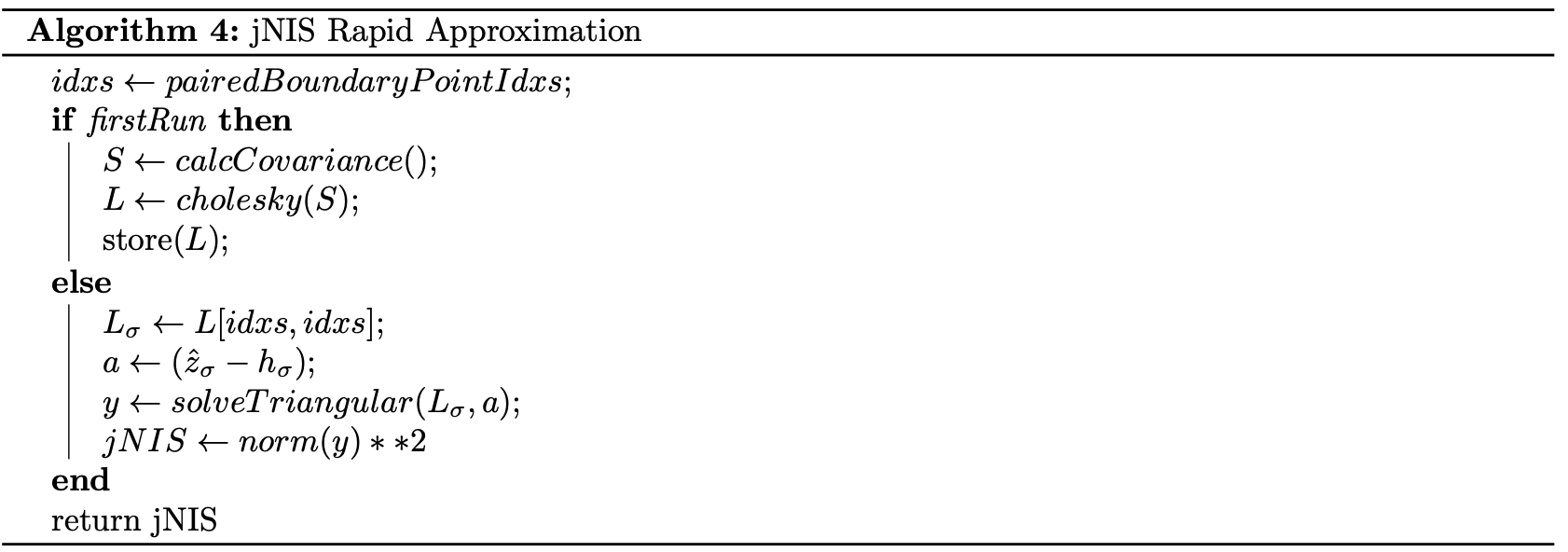
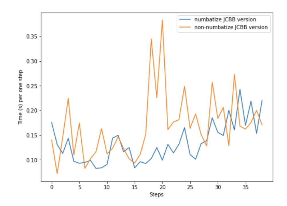
While the resulting jNIS is not completely accurate, as the inverse of portions of the matrix S cannot be completely accurately determined by taking rows and columns from its cholesky, we find that the speed increase (around 10x) yielded by using this approximation exceeds the resulting loss of accuracy. To further improve the speed of JCBB, we wrote a version of it using Numba. We find that this sped up the implementation by around 1.5x ˆahowever, on certain frames, the algorithm can slow down quite a bit. Below is a plot of the loop run times taken from the two systems (the non-Numba JCBB, and the numba JCBB):

Lastly, we attempted to remove the JCBB entirely from the algorithm, by replacing it with a simple algorithm that minimizes the joint distance between two sets of points, and rejects pairings that are too far apart. In practice, we find that this implementation does not generate good associations, causing rapid divergence in the algorithm output.

Transformation Estimation

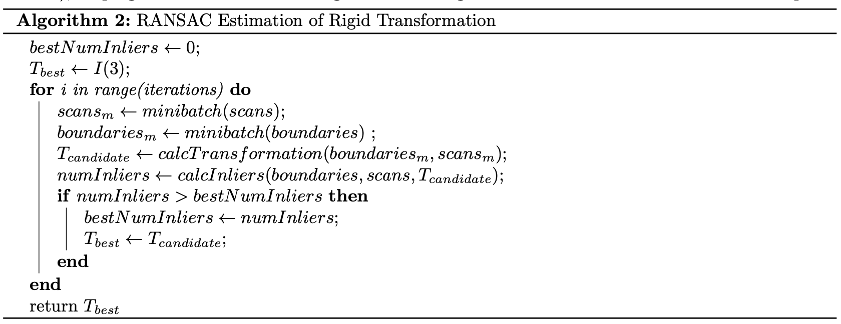
Fine association outputs a set of paired scan points and currently estimated boundary points. These pairs are used to update the hidden state of our tracks. To do this, we diverge from the paper, and use these pair points to estimate a transformation T between the estimated boundary points and scan points. Given that we know the timestep between observations, we can use T to create a fictious measurement of the track’s position, orientation, and velocity. A rigid body transformation is appropriate in this use-case, as we are designing this system for F1Tenth racing, where the only tracks we will likely encounter are other cars, walls, or cones, all relatively rigid objects. This assumption, however, may not be appropriate if this system were deployed on a vehicle that may observe non-rigid objects like humans or animals. As we are estimating a 2D rigid body transformation, T will simply be a 3x3 matrix that encodes the SE(2) transformation that best maps our scan points to our estimated boundary points. To best estimate this transformation, we can either estimate a least squares solution to calculate the transformation matrix between the entire set of pairs via the Kabsch algorithm, or as a cheaper alternative which performs better when the number of pairs is high, run RANSAC, and compute the transformation matrix for a minibatch of pairs (via Kabsch), keeping the transformation that generates the highest number of inliers on the entire set of pairs.

Once the transformation matrix is estimated, it can be used to approximate the fictious measurement by assuming that the transformation occurred as the track was moving with a constant linear and angular velocity.

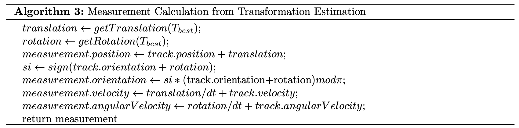
Measurement Model

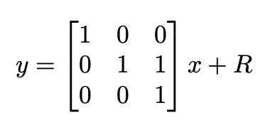
Our “fictious” measurements can be thought of direct observations of the position, velocity, and orientation of tracked objects. These measurements, however, are quite noisy, as data association and transformation estimation both are inherently noisy processes. As such, our measurement model can be thought of as following the below equation, where R is a diagonal noise covariance matrix. In particular, the terms in R associated with velocity (angular and linear) have noise terms that are larger than those associated with position, as velocity estimation is likely to be more noisy that position estimation.

A more robust treatment of the problem may involve looking at the correlation between velocity and position measurements, thus making placing off-diagonal elements in R. Experimentally, however, we find that treating R as a diagonal matrix generates sufficiently accurate tracking.